In a nutshell

Typically, when we investigate the performance of a dose-finding design, we run simulations. If we are comparing several different designs (or variants of a design), we generally run simulations for each candidate design separately. We tend to do this because:

• this is how it is implemented in software;
• different designs are implemented in different packages;
• it might not strike us to do it differently.

However, this is inefficient. By running separate batches of simulations for different designs, we are effectively comparing different designs using different patients. It would be much more efficient to use the same simulated patients on each candidate design. Doing so would reduce the Monte Carlo (random) error inherent in using a finite number of iterations to estimate a limiting value.

The trouble is, dose-finding designs are adaptive, meaning some parameter of the trial (in this instance, the dose delivered and therefore the associated toxicity and efficacy probabilities) is dependent on the outcomes observed in other patients in the trial. Our solution is to effectively simulate all possible binary toxicity (and efficacy) outcomes for a patient in advance by using latent uniform variables on \((0, 1)\). These can be interpreted as patient-level propensities.

To illustrate, imagine a patient’s uniform toxicity propensity is sampled to be \(u_1 = 0.36\). This patient would be regarded as experiencing toxicity when treated at any dose with an associated toxicity probability exceeding 0.36. This allows the same patient to behave consistently when having its dose selected by different designs in simulation. The method works for toxicity-seeking designs like CRM, mTPI and BOIN; and also co-primary efficacy-toxicity designs like EffTox and BOIN12. Full details are in the paper.

The idea of using latent uniform variables to represent propensity to toxicity events has been proposed in different dose-finding contexts (O’Quigley, Paoletti, and Maccario 2002; Cheung 2014).

Code implementation

Our proposal is implemented in v0.1.8 of the escalation package (Brock, Slade, and Sweeting 2023), now uploaded to CRAN. escalation implements many different dose-finding designs with optional behaviour modifiers, making it perfect for comparing the performance of competing designs.

To illustrate, let us reproduce an example from the package vignettes, comparing the behaviour of the perennial 3+3 design and two variants of the CRM in a five-dose scenario. We start by defining the competing designs in a list with convenient names:

library(escalation)

target <- 0.25
skeleton <- c(0.05, 0.1, 0.25, 0.4, 0.6)

designs <- 
  list(
    "3+3" = get_three_plus_three(num_doses = 5),
    "CRM" = get_dfcrm(skeleton = skeleton, target = target) %>%
      stop_at_n(n = 12),
    "Stopping CRM" = get_dfcrm(skeleton = skeleton, target = target) %>%
      stop_at_n(n = 12) %>%
      stop_when_too_toxic(dose = 1, tox_threshold = 0.35, confidence = 0.8)
  )

Here we will compare three designs:

• 3+3;
• CRM without a toxicity stopping rule;
• and an otherwise identical CRM design with a toxicity stopping rule.

The names we provide will be reused.

For illustration we use only a modest number of replicates. Feel free to investigate more replicates yourself. We compare different designs using the simulate_compare function:

num_sims <- 100
true_prob_tox <- c(0.12, 0.27, 0.44, 0.53, 0.57)

sims <- simulate_compare(
  designs, 
  num_sims = num_sims, 
  true_prob_tox = true_prob_tox
)

## Running 3+3 
## Running CRM 
## Running Stopping CRM

We provide a convenient function to quickly visualise how the probability of selecting each dose in each design evolved as the simulations progressed. The dose-levels are represented in the columns of this plot:

convergence_plot(sims)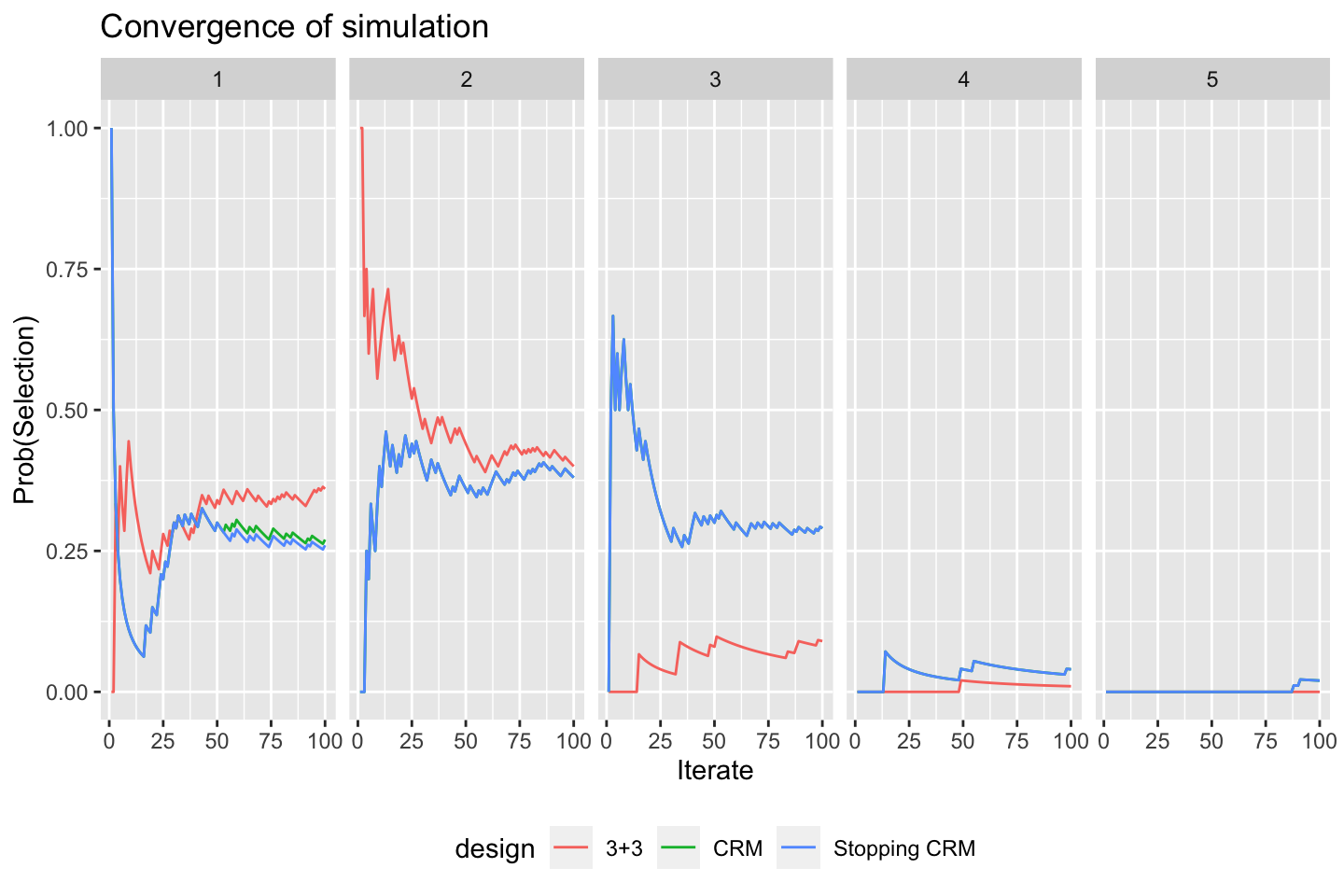

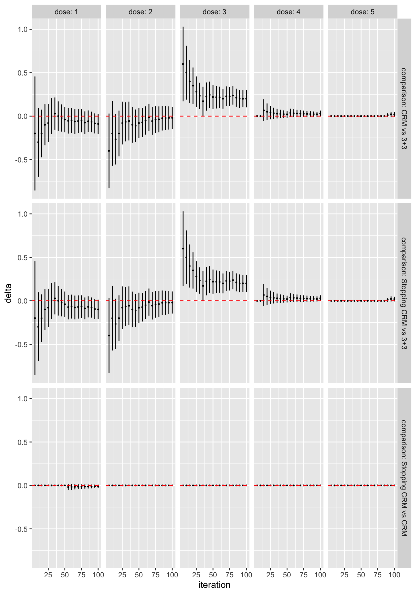
We can see immediately, for instance, that the designs generally agree that dose 2 is the best MTD candidate, and that the CRM designs are more likely to recommend doses 3 and 4. The differences between the two CRM variants are very small. We can be more precise by formally contrasting the probability of selecting each dose for each pair of designs:

library(dplyr)
library(ggplot2)

as_tibble(sims) %>% 
  filter(n %% 5 == 0) %>%
  ggplot(aes(x = n, y = delta)) +
  geom_point(size = 0.4) +
  geom_linerange(aes(ymin = delta_l, ymax = delta_u)) +
  geom_hline(yintercept = 0, linetype = "dashed", col = "red") +
  labs(x = "iteration") +
  facet_grid(comparison ~ dose,
             labeller = labeller(
               .rows = label_both,
               .cols = label_both)
  )

All the work above is done by as_tibble(sims). The rest of the code is just plotting. The error bars here reflect 95% symmetric asymptotic normal confidence intervals. Change the alpha = 0.05 parameter when calling as_tibble(sims) to get confident intervals for a different significance level.

We see that, even with the very small sample size of 50 simulated trials, the CRM designs are significantly more likely to recommend dose 3 than the 3+3 design. In contrast, in this scenario there is very little difference at all between the two CRM variants.

We also provide functions to get and set the patient-level propensities, allowing comparison and reproduction in other software packages. Check out the “Comparing dose-escalation designs by simulation” vignette on the CRAN package page and the package documentation site.