Simulation or enumeration with dose-finding designs?

Introduction

If operating performance of a dose-finding clinical trial design is sought, it is practically guaranteed that this will be by computer simulation. In a dose-finding simulation, a dose is initially selected and toxicity (and perhaps also efficacy) outcomes are sampled according to some assumed true event probabilities to generate data for some imaginary patients. The model is fit to the data and the subsequent dose recommendation is given to the next group of imaginary patients. This iterative and adaptive process continues to conduct a virtual trial. In this manner, many virtual trials are run to inform the trialists of the operating performance of the design.

However, simulating random virtual trials is not the only way to measure operating performance. Richard McElreath said:

If there’s a random way to do something, there’s usually a less random way that is both better and requires more thought.

In dose-finding trials, a less random method is to calculate each trial path using brute force.

Simple example

I demonstrated dose paths (Yap et al. 2017; Brock et al. 2017) in a recent post using the escalation package. Let us walk through a simple example to see how dose-paths and simulation can be used to calculate operating characteristics for a dose-finding trial design.

We load the escalation package:

library(escalation)

## Loading required package: magrittr

For the sake of illustration, let us use:

• a continual reassessment method (CRM) design
• in a three-dose setting
• to target a toxicity rate of 25%
• with a dose-toxicity skeleton that anticipates the middle dose is the sought dose:

target <- 0.25
skeleton <- dfcrm::getprior(0.1, target = target, nu = 2, nlevel = 3)

model <- get_dfcrm(skeleton = skeleton, target = target) %>% 
        stop_at_n(n = 6)

We told the model above to stop when the total sample size reached six patients. Obviously, real trials would generally use larger sample sizes, but six patients will be enough for our illustrative example.

Let us start the trial at the second dose and calculate all possible dose paths for two cohorts of three patients:

paths <- model %>% get_dose_paths(cohort_sizes = rep(3, 2), next_dose = 2)

Viewing the paths makes clear that the decision space is finite and tractable to exact calculation of probabilities:

graph_paths(paths)

Our first instinct might tell us that there are lots of terminal nodes that recommend dose 1 and relatively few that recommend dose 3. We might then infer that selecting dose 1 is likely. In fact, if the true toxicity probabilities at the three doses are (10%, 17%, 25%), we can calculate the exact operating performance:

probs <- c(0.10, 0.17, 0.25)
cdp <- paths %>% calculate_probabilities(true_prob_tox = probs)
prob_recommend(cdp)

##    NoDose         1         2         3 
## 0.0000000 0.1128170 0.4047377 0.4824453

to learn that there is a 40.5% chance that the second dose will be recommended, and a 48.2% chance that the third dose will be recommended.

The object name cdp stands for crystallised dose paths, my name for paths that have associated exact probabilities. Simply printing the object to the console:

cdp

## Number of nodes: 21 
## Number of terminal nodes: 16 
## 
## Number of doses: 3 
## 
## True probability of toxicity:
##    1    2    3 
## 0.10 0.17 0.25 
## 
## Probability of recommendation:
## NoDose      1      2      3 
##  0.000  0.113  0.405  0.482 
## 
## Probability of continuance:
## [1] 0
## 
## Probability of administration:
##      1      2      3 
## 0.0384 0.6757 0.2859 
## 
## Expected sample size:
## [1] 6
## 
## Expected total toxicities:
## [1] 1.141085

confirms the recommendation probabilities and many other statistics.

The more common way to estimate dose-finding design performance is via simulation. escalation supports simulation too:

sims100 <- model %>% 
  simulate_trials(num_sims = 100, true_prob_tox = probs, next_dose = 2)

sims1000 <- model %>% 
  simulate_trials(num_sims = 1000, true_prob_tox = probs, next_dose = 2)

These, too, will estimate the probability that each dose will be recommended when the trial is done:

prob_recommend(sims100)

## NoDose      1      2      3 
##   0.00   0.15   0.40   0.45

prob_recommend(sims1000)

## NoDose      1      2      3 
##  0.000  0.112  0.420  0.468

However, the inferences from the simulations are subject to Monte Carlo error because we have used a finite number of samples to estimate an unknown probability. If we collate the inferences from the dose-paths and simulations:

library(tibble)
library(dplyr)

trial_inference <- function(x, n) {
  dose_labs <- c('NoDose', dose_indices(x))
  tibble(Dose = dose_labs, ProbRecommend = prob_recommend(x), N = n) %>% 
    mutate(
      ProbRecommendSE = sqrt(ProbRecommend * (1 - ProbRecommend) / N),
      ProbRecommendL = ProbRecommend - 2 * ProbRecommendSE,
      ProbRecommendU = ProbRecommend + 2 * ProbRecommendSE
    )
}

inference <- bind_rows(
  trial_inference(cdp, n = Inf) %>% mutate(Method = 'Exact'),
  trial_inference(sims100, n = 100) %>% mutate(Method = 'Sims (N=100)'),
  trial_inference(sims1000, n = 1000) %>% mutate(Method = 'Sims (N=1000)'),
) 

we see the extent and effect of that estimation error:

library(ggplot2)
inference %>% 
  ggplot(aes(x = Dose, y = ProbRecommend, col = Method)) + 
  geom_point(position = position_dodge(width = 0.3)) + 
  geom_errorbar(aes(ymin = ProbRecommendL, ymax = ProbRecommendU), 
                width = 0.1, position = position_dodge(width = 0.3))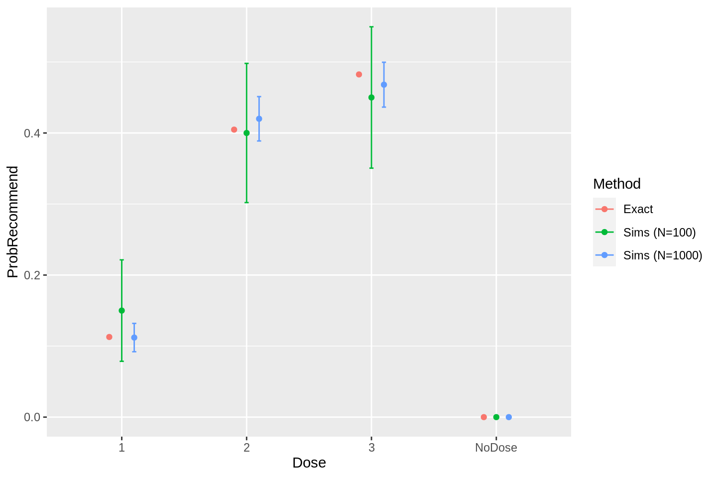

As we might anticipate, the simulation method is hopelessly imprecise with \(N=100\) iterations. In contrast the simulations with \(N=1000\) iterations are fairly precise.

Each simulated trial required that the dose selection model be fit twice, once at the end of each of the two cohorts. A simulation study with 1000 iterations thus required 2000 model fits. We might justifiably conclude that fairly precise is a comparatively bad return on 2000 model invocations when the exact inferences from the dose paths required precisely 21 model fits, one for each of the nodes in the graph above.

Dose paths are more precise than simulations because they are free from the Monte Carlo error that clouds inferences from simulations. In this toy scenario, the paths method was also vastly more efficient, requiring only a small fraction of the model fits.

However, this contrived example is unlikely to be representative of real trial scenarios, where we would expect much higher sample sizes. This invites the question, how far can the dose paths method be taken? When does it become more efficient to run simulations than attempting a brute force calculation?

Calculating paths at scale

Contrasting the computational efficiency of dose paths and simulations requires calculating the number of model invocations expected by each.

For simulations, the arithmetic is simple. Investigating a dose-finding trial of \(M\) cohorts in a single scenario using a simulation study with \(N\) replicates requires \(MN\) model invocations. For example, a trial of \(n=30\) patients evaluated in 10 cohorts requires 10 model invocations, so 1000 simulated replicates requires \(10 \times 1000 = 10000\) model fits in total.

In a dose paths analysis, the model must be fit once for each node in the graph. The number of nodes in a dose paths analysis is slightly more complex to calculate (but only slightly). Let \(k\) be the number of distinct outcomes a single patient may experience. In a phase I trial using the CRM, each patient may experience toxicity (T) or no toxicity (N), so \(k= 2\). The number of outcome combinations in a cohort of \(m\) patients is

\[ \frac{(m + k - 1)!}{m! (k - 1)!} \].

For instance, a cohort of three patients has four possible outcomes: NNN, NNT, NTT, or TTT. The formula above gives \((3 + 2 - 1)! / 3! (2 - 1)! = 4\).

That is the number of outcomes of a single cohort. The number of nodes at depth \(i\) in a graph of dose paths is equal to the number of nodes at depth \(i-1\) multiplied by the number of cohort outcomes at depth \(i\). There is always one node at depth 1 at the centre of the graph. For a cohort of three in a CRM trial, we saw above that there are four possible outcomes. Thus, at depth 2, there are 4 nodes and at depth 2 there are 16 nodes, etc.

Naturally, the cohort sizes may be irregular. In general, the number of nodes at depth \(I\) for cohort sizes \((m_1, ..., m_I)\) is

\[ \prod_{i=1}^I \frac{(m_i + k - 1)!}{m_i! (k - 1)!} \].

Fortunately, there is a function in escalation that calculates the number of nodes in a dose paths analysis. Our simple example with \(n=6\) patients conducted in two cohorts of three has:

num_dose_path_nodes(num_patient_outcomes = 2, cohort_sizes = c(3, 3))

## [1]  1  4 16

nodes at depths, 1, 2, and 3, respectively. The total number of model invocations is the total number of nodes, which is 21, as required.

We can use the function to calculate the number of nodes in an \(n=30\) trial with 10 cohorts of three patients:

n <- num_dose_path_nodes(num_patient_outcomes = 2, cohort_sizes = rep(3, 10))
n

##  [1]       1       4      16      64     256    1024    4096   16384   65536
## [10]  262144 1048576

The number of nodes increases exponentially in graph depth. The total number of model fits is:

sum(n)

## [1] 1398101

1.4m model fits is a substantial computational burden.

Clearly dose number of nodes has increased dramatically as the number of cohorts has increased. Let’s calculate the number of nodes contained in dose-paths of \(M\) cohorts of 3, for increasing values of M:

cohort_size <- 3
num_cohorts <- c(2, 3, 4, 5, 6, 7, 8, 9, 10) %>% as.integer()

library(purrr)
num_model_fits <- map_int(
  num_cohorts, 
  ~ num_dose_path_nodes(num_patient_outcomes = 2, 
                        cohort_sizes = rep(cohort_size, .x)) %>% sum()
)

num_model_fits

## [1]      21      85     341    1365    5461   21845   87381  349525 1398101

THese numbers are the total number of nodes. The final value confirms that roughly 1.4m nodes feature in a graph of paths for eight cohorts of 3 patients. Let’s view those numbers of model invocations alongside the equivalent for simulations with \(N=1000\) and \(10000\) replicates:

bind_rows(
  tibble(NumCohorts = num_cohorts,
         NumModelFits = num_model_fits,
         Method = 'Paths'),
  tibble(NumCohorts = num_cohorts,
         NumModelFits = 1000 * num_cohorts,
         Method = 'Sims (N=1000)'),
  tibble(NumCohorts = num_cohorts,
         NumModelFits = 10000 * num_cohorts,
         Method = 'Sims (N=10000)'),
) %>% 
  ggplot(aes(x = NumCohorts, y = NumModelFits, col = Method)) + 
  geom_point() + 
  geom_line() + 
  scale_y_log10() + 
  labs(y = 'Number of model fits', x = 'Number of cohorts of 3 patients',
       title = 'Computational burden of dose paths and simulation')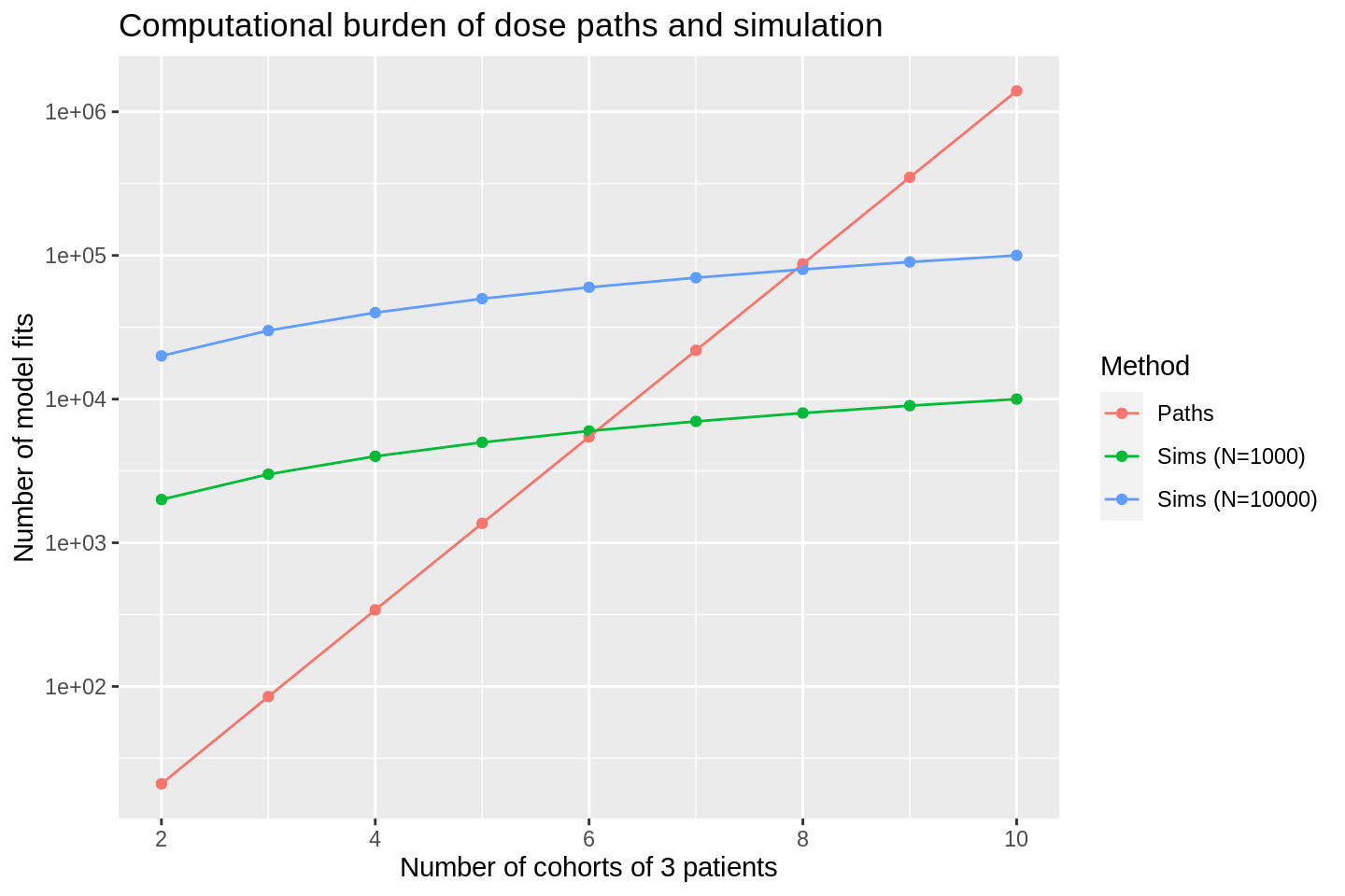

The \(y\)-axis on the plot above is on the log-scale. We see that the number of model fits in the dose paths analysis increases exponentially in the number of cohorts, as expected. In contrast, the number of model fits required by simulations increases linearly in the number of cohorts, generally from a much higher base. The result is that the paths analysis is more computationally efficient than simulations:

• with \(N=1000\) iterations when there are fewer than 6 cohorts of 3;
• with \(N=10000\) iterations when there are fewer than 8 cohorts of 3.

Perhaps we do not plan to use cohorts, intending instead to update the dose recommendation after each patient. We can calculate the computational burdens in this situation:

cohort_size <- 1
num_cohorts <- seq(from = 1, to = 30, by = 1)

num_model_fits <- map_int(
  num_cohorts, 
  ~ num_dose_path_nodes(num_patient_outcomes = 2, 
                        cohort_sizes = rep(cohort_size, .x)) %>% sum()
)

bind_rows(
  tibble(NumCohorts = num_cohorts,
         NumModelFits = num_model_fits,
         Method = 'Paths'),
  tibble(NumCohorts = num_cohorts,
         NumModelFits = 1000 * num_cohorts,
         Method = 'Sims (N=1000)'),
  tibble(NumCohorts = num_cohorts,
         NumModelFits = 10000 * num_cohorts,
         Method = 'Sims (N=10000)'),
) %>% 
  ggplot(aes(x = NumCohorts, y = NumModelFits, col = Method)) + 
  geom_point() + 
  geom_line() + 
  scale_y_log10() + 
  labs(y = 'Number of model fits', x = 'Number of patients',
       title = 'Computational burden of dose paths and simulation')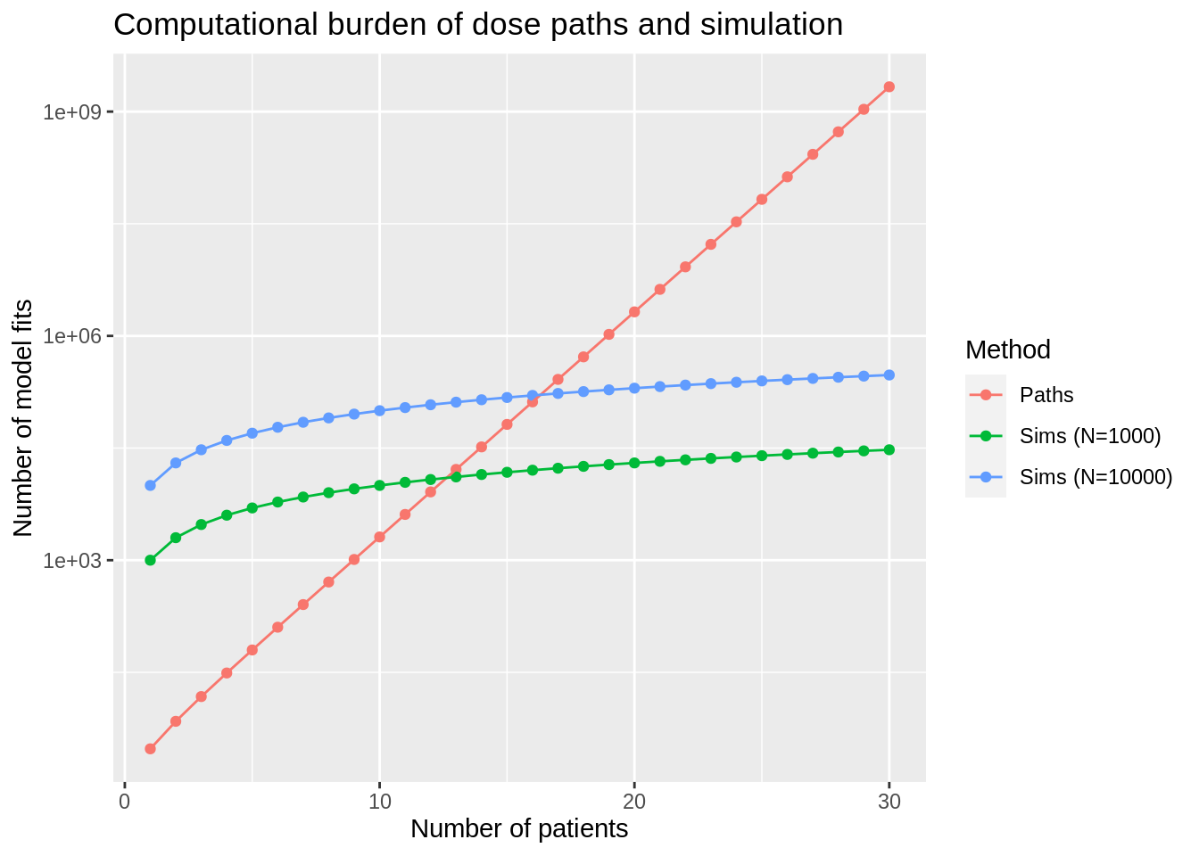

Again, we see that paths are much more efficient for low sample sizes, but sample sizes in excess of 12 - 16 patients favour simulation.

Assuming that dose-finding trials generally have sample sizes of 20-40 patients, that would seem to suggest that simulations clearly vanquish dose-paths for practical use. However, there is one last major consideration to understand.

Conclusion

The number of nodes in a graph of dose paths increases exponentially in the number of cohorts. For 10 cohorts of three patients, approximately 10 times as many model fits are required in dose paths compared to simulations with \(N = 10000\) replicates (recall that the \(y\)-axes above are logarithmic). That is, we expect simulations to be computationally cheaper here if fewer than 10 scenarios are investigated. When the models are evaluated after each patient, dose-paths using \(n=30\) patients require more than \(10^3 = 1000\) times the number of model fits. Simulations are clearly preferable here.

However, we know that dose-paths are more precise. Unlike the simulation method, inferences from dose paths are exact because they are free from Monte Carlo error.

When investigating the operating performance of a clinical trial design, researchers spend computer time to increase certainty. When deciding whether to perform inference via dose paths or simulation, I propose there are three situations:

1. In trials with a small number of cohorts, dose-paths will be both faster and more precise and should naturally be the preferred method for inference.
2. In trials with a modest number of cohorts and many scenarios to analyse, dose-paths will have a similar total computational burden to simulations. In these situations, the extra precision of dose-paths will make them preferable.
3. Finally there will be trials with a high number of cohorts where dose-paths are simply infeasible to calculate. Here, simulations will be preferred.

A way to investgate the value of the two methods in practice is, ironically, a simulation study. This would require plausible assumptions on the number of model fits that should be expected in a trial and how many scenarios would be used to evaluate designs. That feels like it needs a review of the literature but it will have to wait because today I am out of time.

References

Brock, Kristian, Lucinda Billingham, Mhairi Copland, Shamyla Siddique, Mirjana Sirovica, and Christina Yap. 2017. “Implementing the EffTox Dose-Finding Design in the Matchpoint Trial.” BMC Medical Research Methodology 17 (1): 112. https://doi.org/10.1186/s12874-017-0381-x.
Wheeler, Graham M., Adrian P. Mander, Alun Bedding, Kristian Brock, Victoria Cornelius, Andrew P. Grieve, Thomas Jaki, et al. 2019. “How to Design a Dose-Finding Study Using the Continual Reassessment Method.” BMC Medical Research Methodology 19 (1). https://doi.org/10.1186/s12874-018-0638-z.
Yap, Christina, Lucinda J. Billingham, Ying Kuen Cheung, Charlie Craddock, and John O’Quigley. 2017. “Dose Transition Pathways: The Missing Link Between Complex Dose-Finding Designs and Simple Decision-Making.” Clinical Cancer Research 23 (24): 7440–7. https://doi.org/10.1158/1078-0432.CCR-17-0582.
)
Kristian Brock
Statistical Consultant
I am a clinical trial methodology statistician that likes to use Bayesian statistics.