Fitting the Emax Model in R
Emax is an awesome, flexible non-linear model for estimating dose-response curves. Come learn how to fit it in R.
 Photo by adrian on Unsplash
Introduction
Let’s say we have some outcomes observed at different doses or exposures of some intervention. Those data might look like this:
library(ggplot2)
library(dplyr)

df <- tibble(
  Exposure = c(10, 25, 50, 75, 100, 150, 300, 400),
  Response = c(0.03, 0.04, 0.15, 0.12, 0.25, 0.43, 0.54, 0.47)
)

df %>%
  ggplot(aes(x = Exposure, y = Response)) +
  geom_point()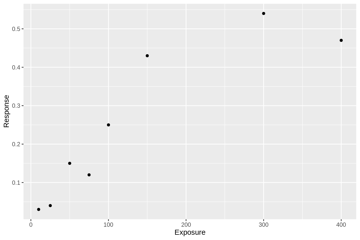
Exposure-response relationships are incredibly common in medical research. They do not just arise in phase I trials.
The response variable could be interpreted as:
- the average level of target inhibition;
- the average concentration in serum;
- the percentage of subjects in a sample experiencing an event.
Likewise, the exposure variable could be interpreted as:
- the prevalence of some characteristic in a population;
- time spent in a certain state;
- the quantity of molecule popped into a patient’s mouth.
So how would we analyse data like this? An ordinary linear model looks a bit of a stretch because the response variable appears to stop increasing at high exposures. A generalised linear model (GLM) might be a fruitful approach.
Here is a logit model fit to the data:
library(broom)

df %>%
  glm(data = ., formula = Response ~ Exposure, family = binomial('logit')) %>%
  augment() %>%
  mutate(Response = gtools::inv.logit(.fitted)) %>%
  ggplot(aes(x = Exposure, y = Response)) +
  geom_line() +
  geom_point(data = df)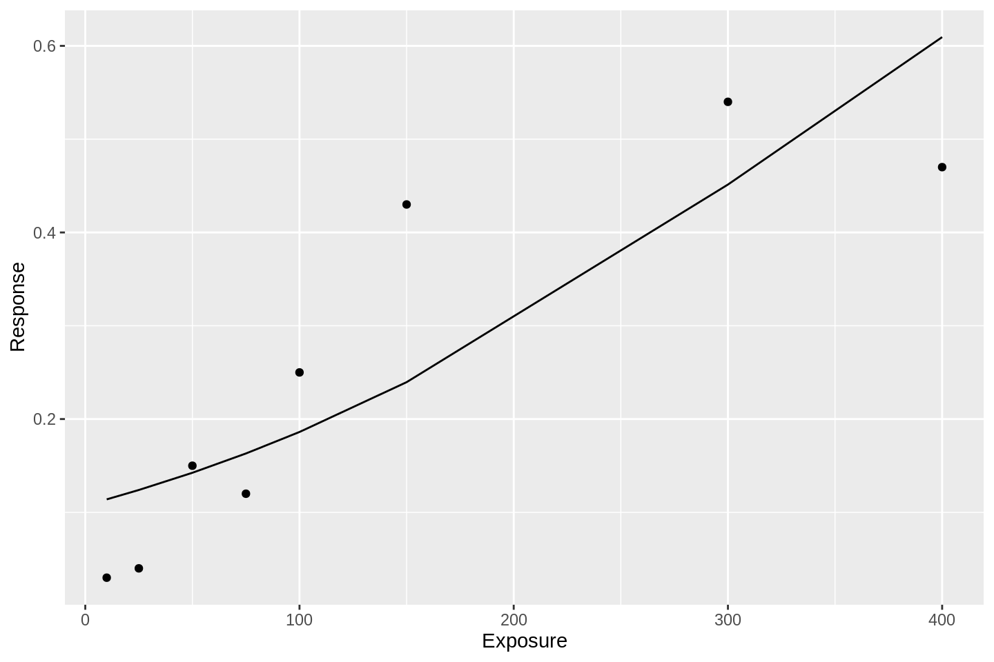
and here is a probit model:
df %>%
  glm(data = ., formula = Response ~ Exposure, family = binomial('probit')) %>%
  augment() %>%
  mutate(Response = gtools::inv.logit(.fitted)) %>%
  ggplot(aes(x = Exposure, y = Response)) +
  geom_line() +
  geom_point(data = df)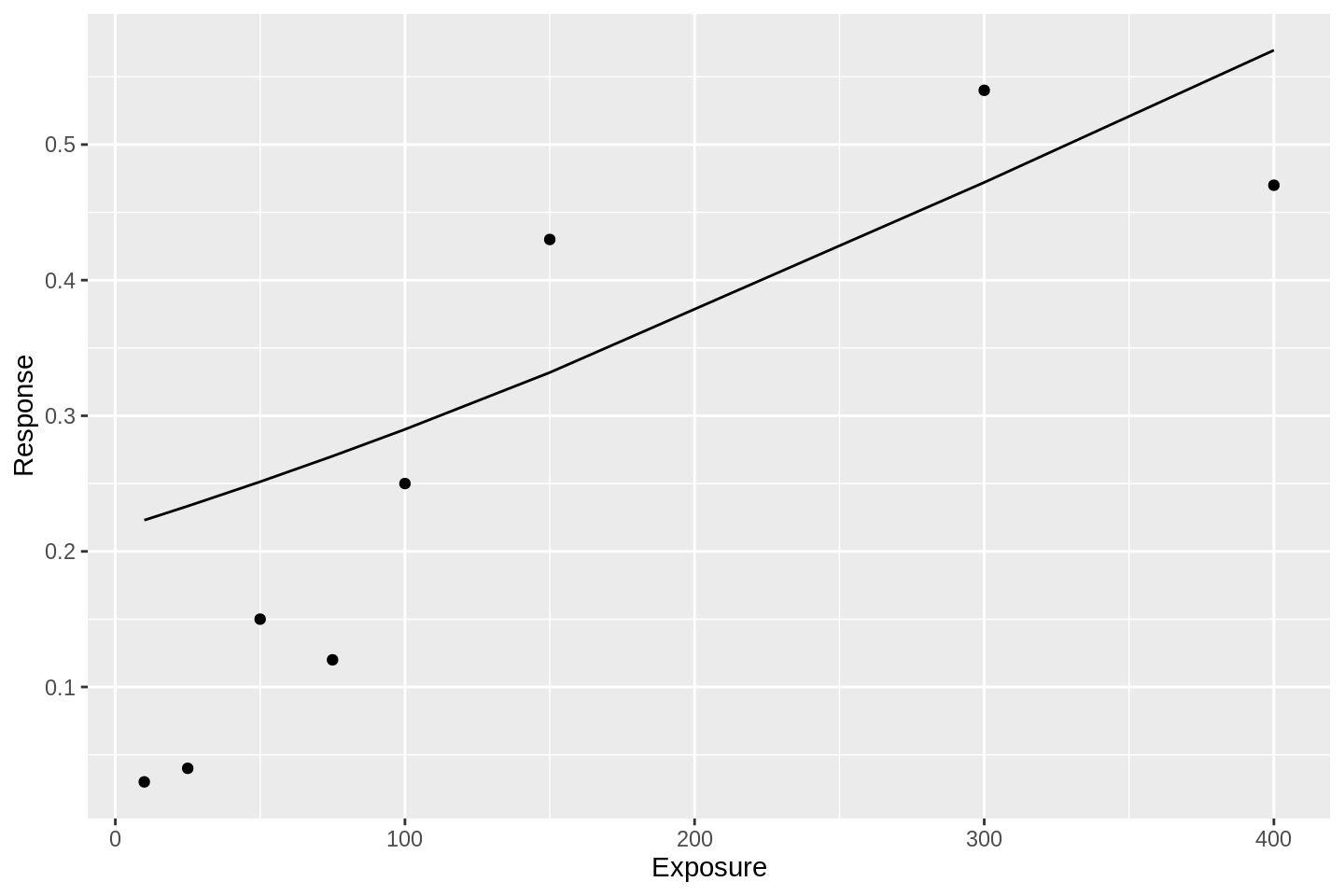
These fits are awful. Both of these GLM approaches suffer from the same simple problem; they assume that the event probability tends to 1 as the linear predictor tends to infinity. Put another way, there is no way for the response curve to asymptote to some value other than 1.0. This bakes into the analysis that an event probability of 1.0 is not only possible, but guaranteed, given high enough exposure. In many situations, this assumption is inappropriate.
So what might we do instead?
The Emax Model
Emax is a non-linear model for estimating dose-response curves.
The general model form is:
\[ R_i = E_o + \frac{D_i^N \times E_{max}}{D_i^N + {ED}_{50}^N}\]
where:
- \(R_i\) is the response for experimental unit \(i\);
- \(D_i\) is the exposure (or dose) of experimental unit \(i\);
- \(E_0\) is the expected response when exposure is zero, or the zero-dose effect, or the basal effect;
- \(E_{max}\) is the maximum effect attributable to exposure;
- \(ED_{50}\) is the exposure that produces half of \(E_{max}\);
- \(N > 0\) is the slope factor, determining the steepness of the dose-response curve.
Macdougall (2006) gives a fantastic introduction to the method, providing excellent interpretation of the parameters and summaries of the main model extensions. We have borrowed here their notation and elementary explanation of model terms.
The model variant above is called the sigmoidal Emax model. The variant with \(N\) fixed to take the value 1 is called the hyperbolic model.
Fitting this model to some data means estimating values for the free parameters, \(E_0, E_{max}, ED_{50}\), and possibly \(N\), conditional on the observed \(R_i\) and \(D_i\).
Fortunately, there are packages in R that will fit this model. We introduce maximum likelihood and Bayesian approaches below.
Maximum likelihood methods
Bornkamp (2019) provides a function in the DoseFinding package for fitting both the hyperbolic and sigmoidal model variants.
We demonstrate first the hyperbolic approach, fitting it to our manufactured dataset:
library(DoseFinding)

emax0 <- fitMod(Exposure, Response, data = df,  model = "emax")
plot(emax0)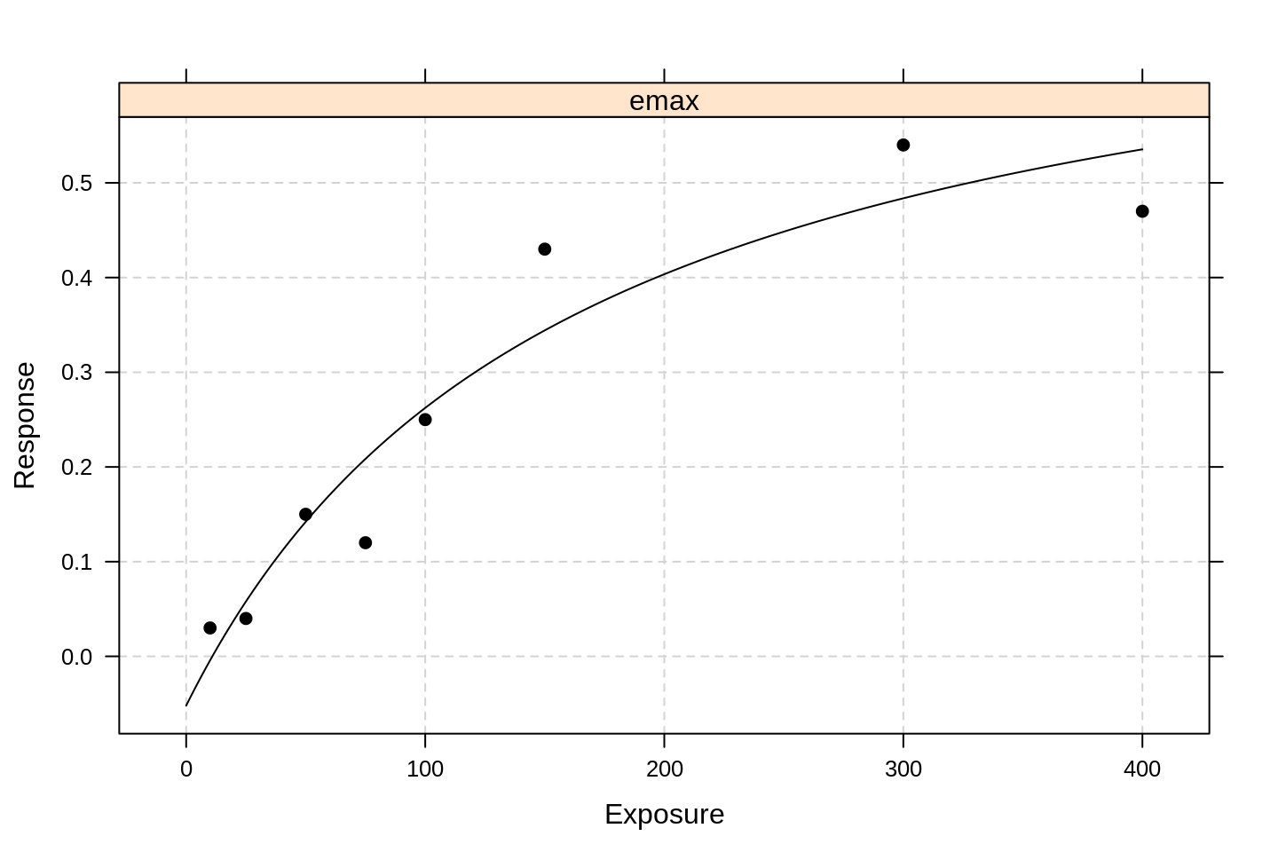
By default, the package uses lattice-type graphics.
We see that the model fit is much better than the GLM approaches above.
To see the estimated parameters, we run:
summary(emax0)## Dose Response Model
##
## Model: emax
## Fit-type: normal
##
## Residuals:
## Min 1Q Median 3Q Max
## -0.08579 -0.03974 0.00223 0.02980 0.08854
##
## Coefficients with approx. stand. error:
## Estimate Std. Error
## e0 -0.052 0.079
## eMax 0.827 0.172
## ed50 162.962 117.031
##
## Residual standard error: 0.0698
## Degrees of freedom: 5We now fit the sigmoidal model.
This simply involves calling the same function with a different model parameter:
emax1 <- fitMod(Exposure, Response, data = df,  model = "sigEmax")
plot(emax1)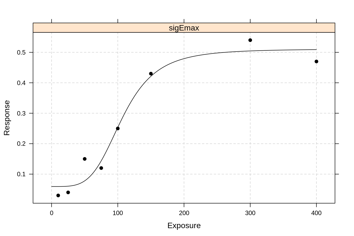
It is clear that the extra parameter dramatically improves the model fit. Glimpsing the parameter values:
summary(emax1)## Dose Response Model
##
## Model: sigEmax
## Fit-type: normal
##
## Residuals:
## Min 1Q Median 3Q Max
## -0.0721 -0.0154 0.0120 0.0251 0.0389
##
## Coefficients with approx. stand. error:
## Estimate Std. Error
## e0 0.0594 0.0324
## eMax 0.4515 0.0535
## ed50 107.0215 11.5670
## h 4.1370 1.6398
##
## Residual standard error: 0.0497
## Degrees of freedom: 4we learn that the \(N\) parameter (which they call h to keep us on our toes) is not particularly consistent with the value 1.
The extra degree of freedom has roughly halved the estimated value of \(E_{max}\) and more than halved the associated standard error.
Bayesian methods
The rstanemax package by Yoshida (2019) implements a Bayesian version of Emax, offloading MCMC sampling to the miracle software Stan (Carpenter et al. 2016).
Fitting the sigmoidal model is as simple as running code like:
library(rstanemax)

stan1 <- stan_emax(Response ~ Exposure, data = df, gamma.fix = NULL,
                   seed = 12345, cores = 4, control = list(adapt_delta = 0.95))
stan1
## Inference for Stan model: emax.
## 4 chains, each with iter=2000; warmup=1000; thin=1;
## post-warmup draws per chain=1000, total post-warmup draws=4000.
##
## mean se_mean sd 2.5% 25% 50% 75% 97.5% n_eff Rhat
## emax 0.51 0.00 0.12 0.35 0.44 0.48 0.55 0.86 681 1
## e0 0.04 0.00 0.04 -0.05 0.02 0.05 0.07 0.12 1409 1
## ec50 122.33 1.76 45.01 81.81 100.91 110.81 124.89 257.70 651 1
## gamma 3.66 0.06 2.03 0.96 2.18 3.32 4.74 8.67 1220 1
## sigma 0.07 0.00 0.03 0.03 0.05 0.06 0.08 0.14 923 1
##
## Samples were drawn using NUTS(diag_e) at Wed May 13 19:15:55 2020.
## For each parameter, n_eff is a crude measure of effective sample size,
## and Rhat is the potential scale reduction factor on split chains (at
## convergence, Rhat=1).The \(N\) parameter in this package is referred to as gamma (still with me?) and the gamma.fix = NULL argument causes the variable to be estimated from the data.
The argument name suggests you can provide your own fixed value - I have not investigated.
To fit the hyperbolic version, you just omit the gamma.fix argument.
We see that there is a little bit of difference in each of the estimated variables but nothing to get alarmed about.
The package also provides a nice way of fetching predicted values:
samp <- rstanemax::posterior_predict(
  stan1, returnType = "tibble",
  newdata = tibble(exposure = seq(0, 400, length.out = 100)))

samp %>% head(10) %>% knitr::kable()| mcmcid | exposure | emax | e0 | ec50 | gamma | sigma | respHat | response |
|---|---|---|---|---|---|---|---|---|
| 100 | 0.000000 | 0.1712489 | 0.0718365 | 89.70576 | 2.741876 | 0.1903292 | 0.07183650 | -0.2860366 |
| 100 | 4.040404 | 0.1712489 | 0.0718365 | 89.70576 | 2.741876 | 0.1903292 | 0.07187133 | 0.3240279 |
| 100 | 8.080808 | 0.1712489 | 0.0718365 | 89.70576 | 2.741876 | 0.1903292 | 0.07206919 | 0.2041787 |
| 100 | 12.121212 | 0.1712489 | 0.0718365 | 89.70576 | 2.741876 | 0.1903292 | 0.07254184 | 0.0818142 |
| 100 | 16.161616 | 0.1712489 | 0.0718365 | 89.70576 | 2.741876 | 0.1903292 | 0.07338111 | -0.0172850 |
| 100 | 20.202020 | 0.1712489 | 0.0718365 | 89.70576 | 2.741876 | 0.1903292 | 0.07466294 | 0.1978203 |
| 100 | 24.242424 | 0.1712489 | 0.0718365 | 89.70576 | 2.741876 | 0.1903292 | 0.07644671 | 0.2342920 |
| 100 | 28.282828 | 0.1712489 | 0.0718365 | 89.70576 | 2.741876 | 0.1903292 | 0.07877353 | 0.0095302 |
| 100 | 32.323232 | 0.1712489 | 0.0718365 | 89.70576 | 2.741876 | 0.1903292 | 0.08166463 | -0.0747148 |
| 100 | 36.363636 | 0.1712489 | 0.0718365 | 89.70576 | 2.741876 | 0.1903292 | 0.08512041 | -0.0137214 |
This facilitates my favourite method of visualising Bayesian model inferences: overplotting dots and lines.
E.g. how does the expected curve look?
samp %>% head(100 * 150) %>%
  rename(Exposure = exposure, Response = respHat) %>%
  ggplot(aes(x = Exposure, y = Response)) +
  geom_point(data = df) +
  geom_line(aes(group = mcmcid), alpha = 0.1, col = 'purple') +
  ylim(0, NA)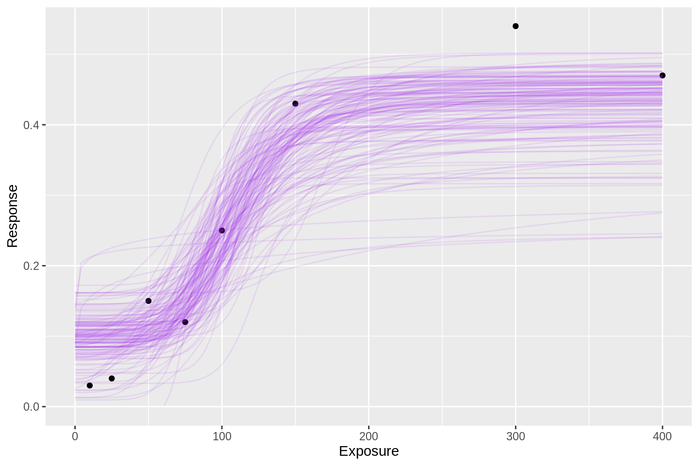
Each of the 150 purple lines above is a candidate for the mean exposure-response curve (or dose-response curve, if you prefer), hence the column name respHat.
The subject-level predictions (i.e. the predictions with added noise) are also available in the samp object via the response column.
For instance, if you wanted to infer on the distribution of responses for a single unit (patient, dog, country, whatever) with given exposure, this is the distribution you would be using:
samp %>% head(100 * 100) %>%
  rename(Exposure = exposure, Response = response) %>%
  ggplot(aes(x = Exposure, y = Response)) +
  geom_point(alpha = 0.1) +
  ylim(0, NA)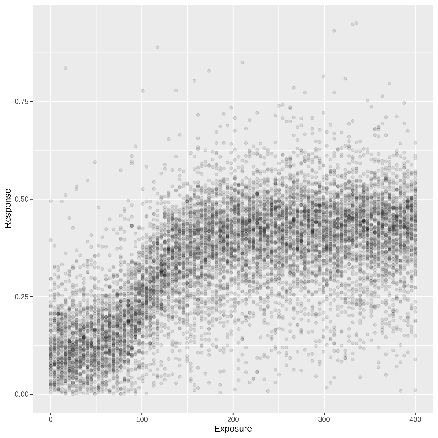
In the plot above, responses are predicted at each of one hundred evenly-spaced exposures. At each exposure, there are 100 points shown - i.e. each vertical tower contains exactly 100 points. Thus, each dot represents a percentile.
That is a bloody nice plot, isn’t it? Time to sign off.
Next steps
In a forthcoming post I will fit the Emax model to outcomes in the dataset of phase I outcomes of Brock et al. (2019) introduced in this post. Til then.
References
Bornkamp, Bjoern. 2019. DoseFinding: Planning and Analyzing Dose Finding Experiments. https://CRAN.R-project.org/package=DoseFinding.
Brock, Kristian, Victoria Homer, Gurjinder Soul, Claire Potter, Cody Chiuzan, and Shing Lee. 2019. “Dose-Level Toxicity and Efficacy Outcomes from Dose-Finding Clinical Trials in Oncology.” https://doi.org/10.25500/edata.bham.00000337.
Carpenter, Bob, Andrew Gelman, Matt Hoffman, Daniel Lee, Ben Goodrich, Michael Betancourt, Marcus A. Brubaker, Peter Li, and Allen Riddell. 2016. “Stan: A Probabilistic Programming Language.” Journal of Statistical Software 76 (Ii): 1–32.
Macdougall, James. 2006. “Analysis of Dose–Response Studies—Emax Model.” In Dose Finding in Drug Development, edited by Naitee Ting, 127–45. New York, NY: Springer New York. https://doi.org/10.1007/0-387-33706-7_9.
Yoshida, Kenta. 2019. Rstanemax: Emax Model Analysis with ’Stan’. https://CRAN.R-project.org/package=rstanemax.
)
Kristian Brock
Statistical Consultant
I am a clinical trial methodology statistician that likes to use Bayesian statistics.