Sample sizes in phase I

Empirically, what sample size is used in dose-escalation trials?

Last updated on Jun 24, 2020 4 min read Research

Project

Introduction

I recently had reason to estimate the average size of a dose-escalation trial. Based on my own experience, my immediate answer was “about 30 patients”. However, using the data of Brock et al. (2019) introduced in this recent post, there is no reason to guess. The dataset contains dose-level outcomes from 122 phase I clinical trial manuscripts reporting results of 139 dose-escalation experiments in cancer between 2008 and 2014.

Perhaps surprisingly, we did not record the sample size of each trial. The focus of the research was not phase I trials per se, but the outcomes seen at individual doses in phase I trials. For that reason, we recorded the number of patients evaluable at each dose for several outcomes, including toxicity and efficacy outcomes. As this post explains, the outcome most commonly reported was incidence of dose-limiting toxicity (DLT), with about 95% of studies reporting dose-level DLT data. Thus, we can derive the number of patients in a dose-escalation study by summing the numbers of patients at each dose.

Empirical sample size of phase I trials

With those caveats out the way, let’s load the data:

source('https://raw.githubusercontent.com/brockk/dosefindingdata/master/Load.R')

and some required packages:

library(dplyr)
library(ggplot2)

and then calculate the number of patients in each study:

dlt_evaluable <- binary_events %>% 
  filter(OutcomeId == 1) %>% # This is DLT
  group_by(Study) %>% 
  summarise(NumPatients = sum(n), NumDoses = n())

We can simply visualise those summarised data:

dlt_evaluable %>% 
  ggplot(aes(x = NumPatients)) + 
  stat_count(aes(y = ..prop..), alpha = 0.5) + 
  geom_density(col = 'blue', size = 1.3) + 
  xlim(0, NA) + 
  labs(x = 'Total sample size', y = 'Proportion')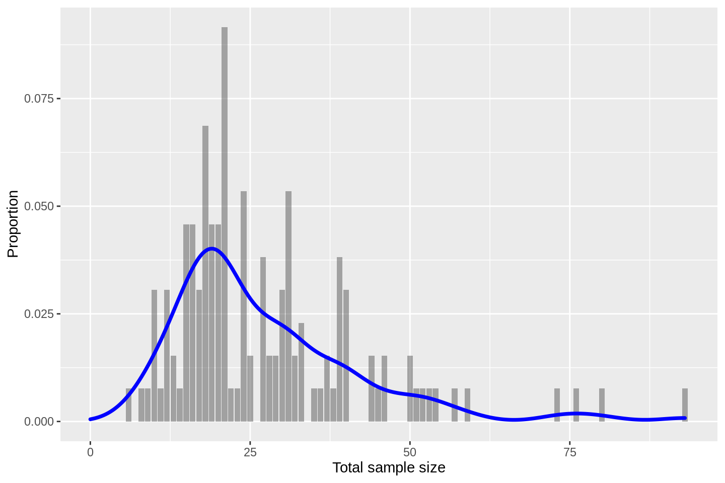

to learn that the modal size is about \(n=20\). The distribution has a pronounced positive skew with a small number of relatively large sample sizes seen.

Calculating summary statistics:

dlt_evaluable %>% 
  pull(NumPatients) %>% 
  summary()

##    Min. 1st Qu.  Median    Mean 3rd Qu.    Max. 
##    6.00   18.00   23.00   27.38   33.00   93.00

we see that the median size is 23 patients with an inter-quartile range of (18, 33). My initial guess of about 30 was a bit toppy.

By drug type

The database also records various descriptive variables about the clinical scenarios. We can, for example, investigate sample size by the type of drug that is having its dose varied.

Let’s do that. First, let us check which treatment types are contained:

dlt_evaluable %>% 
  left_join(studies, by = 'Study') %>%
  count(DoseVaryingTreatmentType) %>% 
  arrange(-n) %>% 
  head(5) %>% knitr::kable(digits = 1)

DoseVaryingTreatmentType	n
Chemotherapy	49
Inhibitor	48
Monoclonal Antibody	8
Chemotherapy + inhibitor	6
Immunomodulatory drug	4

We see that this period yielded trials mostly of chemotherapy and inhibitor drugs. It really only makes sense to summarise sample sizes for those two categories:

dlt_evaluable %>% 
  left_join(studies, by = 'Study') %>%
  filter(DoseVaryingTreatmentType %in% c('Chemotherapy', 'Inhibitor')) %>% 
  ggplot(aes(x = NumPatients)) + 
  stat_count(aes(y = ..prop..), alpha = 0.5) + 
  geom_density(col = 'blue', size = 1.3) + 
  xlim(0, NA) + 
  facet_wrap(~ DoseVaryingTreatmentType, ncol = 1) + 
  labs(x = 'Total sample size', y = 'Proportion')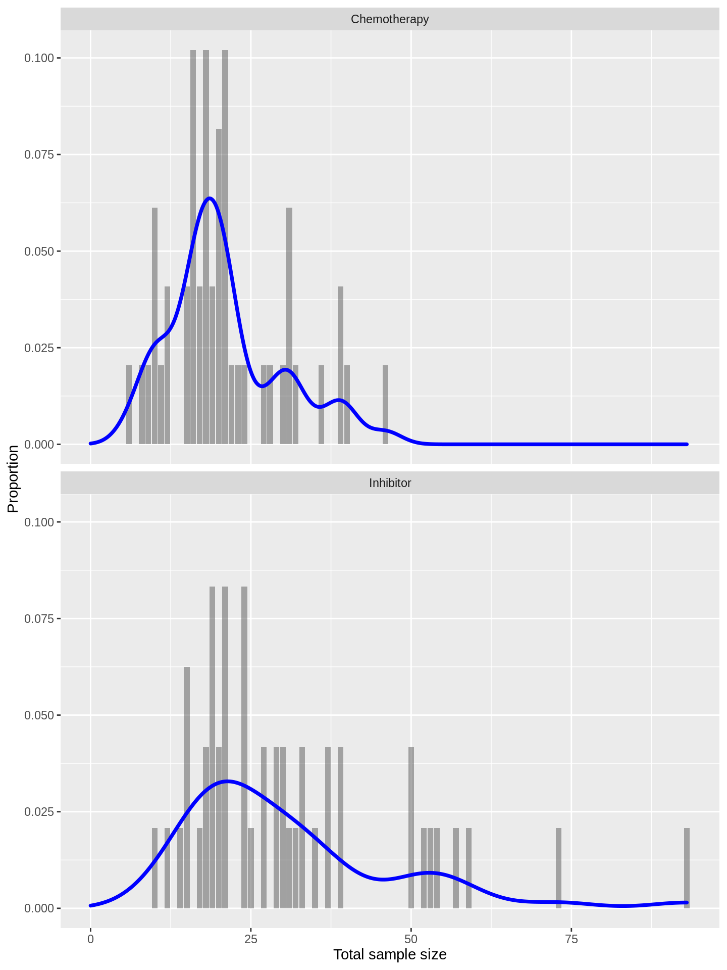

The distributions look fairly exchangeable, suggesting that phase I trials of inhibitors have tended to use similar sizes to those of chemotherapies.

Haematological vs non-haematological

We can instead contrast the sample sizes of trials in haematological and solid tumour (or non-haematological) diseases:

dlt_evaluable %>% 
  left_join(studies, by = 'Study') %>%
  filter(HaemNonhaem %in% c('Haematological', 'NonHaematological')) %>% 
  ggplot(aes(x = NumPatients)) + 
  stat_count(aes(y = ..prop..), alpha = 0.5) + 
  geom_density(col = 'blue', size = 1.3) + 
  xlim(0, NA) + 
  facet_wrap(~ HaemNonhaem, ncol = 1) + 
  labs(x = 'Total sample size', y = 'Proportion')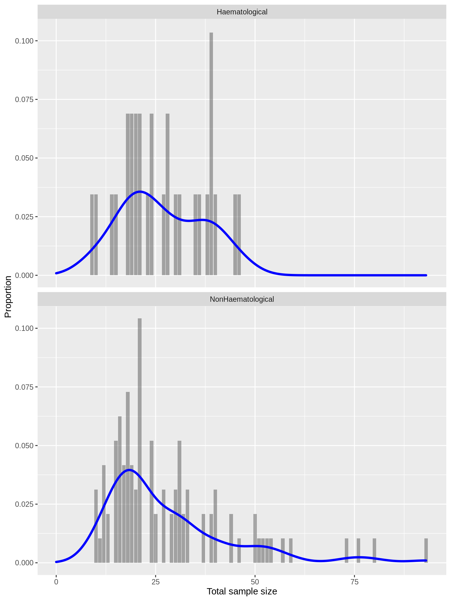

Again, we see that the distributions are largely coincident.

Sample-size per dose investigated

We can plot sample size against the number of dose investigated to learn roughly how many patients are evaluated at each dose:

dlt_evaluable %>% 
  ggplot(aes(x = NumDoses, y = NumPatients)) + 
  geom_point() + 
  geom_smooth(method = 'loess') + 
  xlim(0, NA)

## `geom_smooth()` using formula 'y ~ x'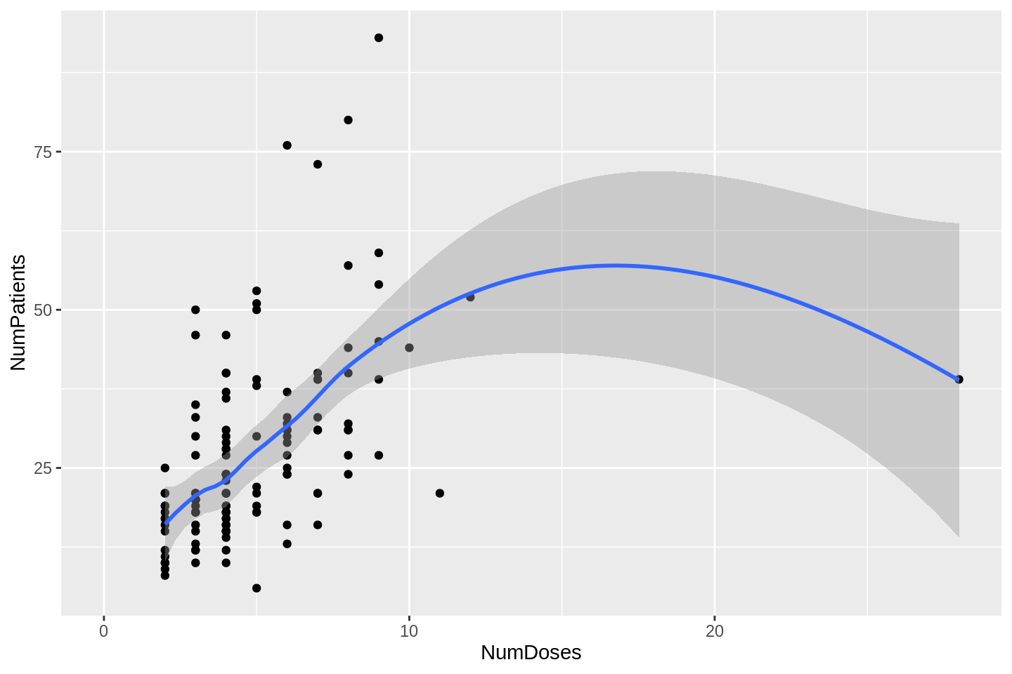

In one particular study, each patient received a different dose. That is the outlier on the right of the plot above. If we exclude that point, we get a better look at the relationship:

dlt_evaluable %>% 
  filter(NumDoses < 20) %>% 
  ggplot(aes(x = NumDoses, y = NumPatients)) + 
  geom_point() + 
  geom_smooth(method = 'loess') + 
  xlim(0, NA)

## `geom_smooth()` using formula 'y ~ x'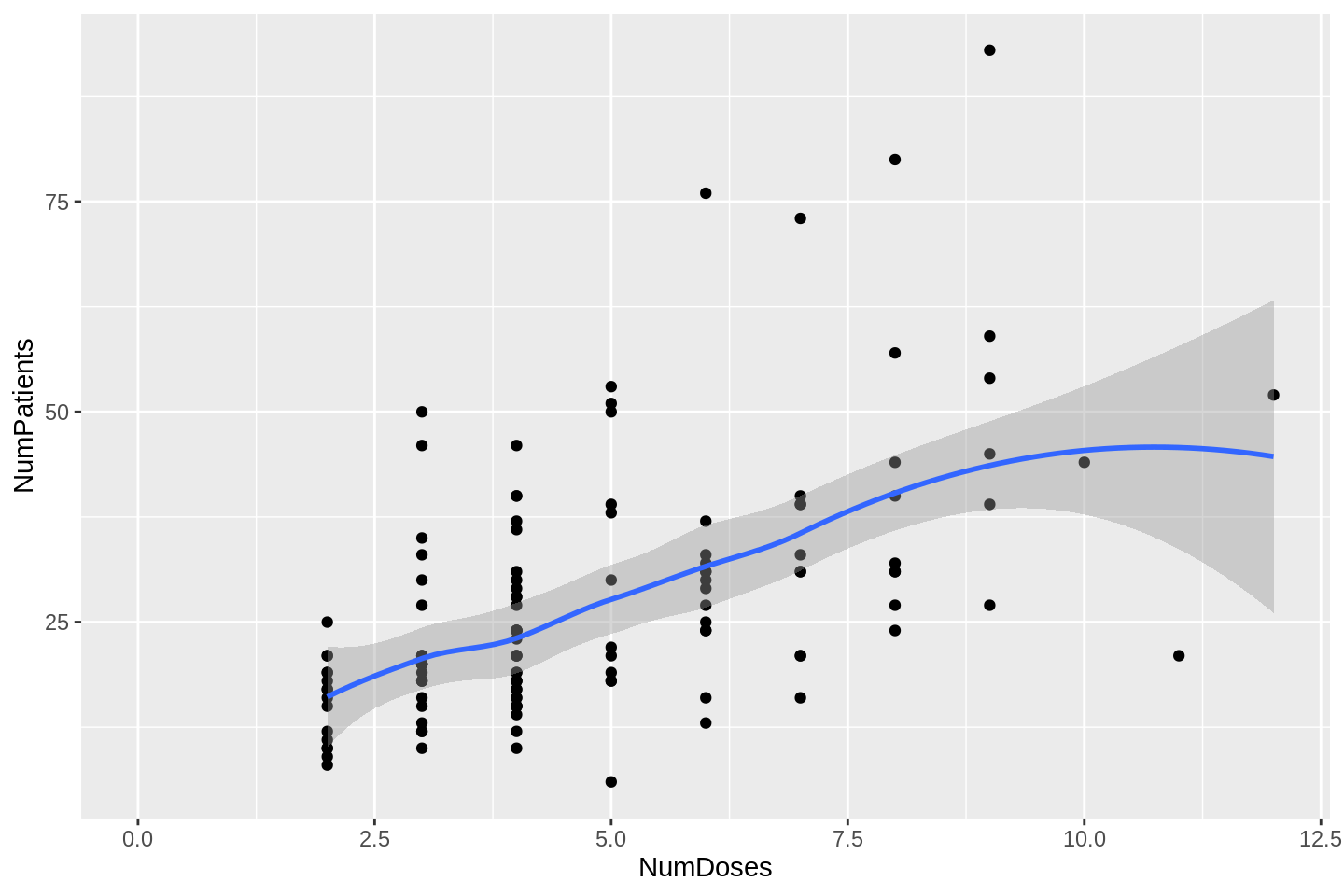

For numbers of doses less than about 10, the aggregate sample size is broadly linear in the number of doses. How many patients per dose?

dlt_evaluable %>% 
  filter(NumDoses < 20) %>% 
  lm(NumPatients ~ NumDoses, data = .) %>% 
  broom::tidy() %>% knitr::kable()

term	estimate	std.error	statistic	p.value
(Intercept)	9.020828	2.6361675	3.421948	0.0008352
NumDoses	3.831117	0.5030493	7.615787	0.0000000

About 4, with (3, 5) being a good working uncertainty interval. That is not to say that phase I trials should be that size, of course! Merely a reflection of what was done, on average, between 2008 and 2014.

References

Brock, Kristian, Victoria Homer, Gurjinder Soul, Claire Potter, Cody Chiuzan, and Shing Lee. 2019. “Dose-Level Toxicity and Efficacy Outcomes from Dose-Finding Clinical Trials in Oncology.” https://doi.org/10.25500/edata.bham.00000337. https://doi.org/10.25500/edata.bham.00000337.

DoseFinding